Reading in Data and Example Analysis

In this exercise, we will learn how to read in data as an object in R, find and load packages into our library, and then re-create Figure 2 from the 2017 paper by Morini et al. paper “Control of white mold of dry bean and residual activity of fungicides applied by chemigation.”

We can use the read.table() function to read these data in to R. It’s important to remember that while in R, these data are simply a copy kept in memory, not on the disk, so we don’t have to worry too much about accidentally deleting the data :).

So, how do we actually USE the read.table() function? A good first step to figuring out how you can use a function is to look at it’s help page. The way you can do that is by typing either help(“function_name”) or ?function_name.

>      # Type ?read.table and answer these three questions:
>      # 
>      # 1. What does it do? (Description)
>      # 2. What are the first three arguments and their defaults? (Usage/Arguments)
>      # 3. What does it return? (Value)

In order to read our data into R, we will need to provide three things:

The path to the data set : Results2017_combined-class.csv
If the first row are column names : yes
The separator for each cell in the data : comma

Now that we have these elements, we can read our data into a variable, which we can call “res” because it is short for “results”. Once we do this, we should check the dimensions to make sure that we have all of the data.

Now we can read in the data and inspect to make sure it is what we expect.

> res <- read.csv("Results2017_combined-class.csv", head = TRUE, stringsAsFactors = FALSE)
> head(res)

  DAI Number Your.name   Area      Treatment Block
1   1      1      Noel 19.808        control     1
2   1      2      Noel  9.371  2.53 mm water     1
3   1      3      Noel  0.000  5.07 mm water     1
4   1      4      Noel  0.531 10.13 mm water     1
5   1      5       Lee  0.000 10.13 mm water     2
6   1      6       Lee 20.914        control     2

> dim(res)

[1] 288   6

This shows the data in columns named DAI, Number, Your.name, Area, and Treatment.

Thinking before doing: Your data and the analysis

The example data presented here were collected by students in the 2017 PLPT802 class and should represent the same data that this year’s class collected. This data consists of six columns of data: DAI, Number, Your.name, Area, Treatment, and Block. With these data, we want to answer the following questions:

Can we convert lesion areas to a measurement that is relative to the control?
What do we want to plot in order to demonstrate the residual disease control over time by treatment?

To answer these questions, we will need to manipulate the layout of the data and will also need to write a function to perform a calculation and then plot the results of the calculations over time. Not all data manipulations will be described in detail here and are shown so that you can re-run this analysis using data collected in class. We will do this using the following four steps:

> #

Create a function
Spread the data in different columns by treatment
Calculate percent disease control
Summarize the average lesion area in a plot

> #
> #

Preparing Data and Packages

We will re-create the figure using three packages dplyr, tidyr, and ggplot2. These packages add flexibility to data and figure manipulations. We will not go into these in detail. Refer to the tab in this website called “Other Exercises” to get started learning more.

> library("dplyr")
> library("tidyr")
> library("ggplot2")

Reordering factors

The factors in the treatments will be out of order when plotting because it’s always alphabetical by default (and 1 comes before 2). Here we are reordering the factors:

> unique(res$Treatment) # The correct order

[1] "control"        "2.53 mm water"  "5.07 mm water"  "10.13 mm water"

> res <- mutate(res, Treatment = factor(Treatment, levels = unique(Treatment)))
> levels(res$Treatment)

[1] "control"        "2.53 mm water"  "5.07 mm water"  "10.13 mm water"

Calculating Percent Disease Control

Percent disease control is “estimated as the difference in lesion area of the control and treatment, divided by lesion area of the control and expressed as percent.” Because we will have to make this calculation many times, it’s best to write a function for it.

Step 1: Create a function

Our function will take in two numbers, the lesion area of the control and the lesion area of the treatment.

> percent_control <- function(control, treatment){
+   res <- (control - treatment)/control # estimate the disease control
+   return(res*100)                      # express as percent
+ }

We can show that this works:

> percent_control(control = 10, treatment = 5)

[1] 50

Step 2: Spread the data in different columns by treatment

Our data were recorded in a “tidy” fashion in which we had one observation per row. In order to calculate the percent control, we’ll need to rehshape our data so that we have one column per treatment such that each row will represent a single block per day after application. We’ll use the tidyr function spread() to do this.

> blocks <- res %>%
+   select(DAI, Block, Treatment, Area) %>% # We don't need name or number here
+   spread(Treatment, Area) # make new columns from treatment, and fill with Area
> blocks

   DAI Block control 2.53 mm water 5.07 mm water 10.13 mm water
1    1     1  19.808         9.371         0.000          0.531
2    1     2  20.914         0.000         0.173          0.000
3    1     3  15.206        21.173         0.000         18.270
4    1     4  11.598         0.000         5.736          9.524
5    1     5   3.034         0.000         0.458          1.943
6    1     6   8.770        12.053        13.148          0.000
7    1     7  12.951         0.000        15.283         14.839
8    1     8  20.537         0.000        12.080          1.737
9    1     9  25.941         0.000         7.428          1.592
10   1    10  22.998         3.106         0.000          7.679
11   1    11  15.302         0.000        20.567          0.000
12   1    12  23.496         0.000        14.778          0.000
13   3     1   4.853        18.860         1.632         10.572
14   3     2  20.540         0.000         5.032          0.000
15   3     3  20.577        13.730         0.000         10.990
16   3     4  20.374         8.404         0.000          0.000
17   3     5  18.757         2.168         0.000          8.969
18   3     6   0.000         9.768         0.000          0.000
19   3     7  21.004         0.000        18.070         18.346
20   3     8  27.562         3.396         3.715          0.000
21   3     9   4.378         0.922         0.000          0.000
22   3    10   5.200         1.206         0.000          0.000
23   3    11   3.249         0.000         0.565          1.558
24   3    12   4.874         0.000         1.989          1.954
25   5     1   4.883         0.043         0.790          0.000
26   5     2   3.056         1.605         3.636          5.114
27   5     3   5.618         3.883         5.844          0.156
28   5     4   6.982         3.231         1.904          3.178
29   5     5   5.009         1.302         1.713          3.706
30   5     6   7.928         0.000         1.283          3.645
31   5     7   3.008         2.018         0.000          2.141
32   5     8   6.897         0.409         2.970          0.308
33   5     9   7.436         3.427         2.257          4.952
34   5    10   3.220         2.375         6.440          5.177
35   5    11   0.216         1.559         3.864          0.000
36   5    12   4.263         0.000         2.708          7.763
37   7     1   9.142         7.791         6.630          5.999
38   7     2   5.434         1.156        10.471          8.931
39   7     3   8.585         0.000         6.271          5.393
40   7     4  10.235         4.716         5.185          6.353
41   7     5  55.971        13.891         1.525         12.636
42   7     6  31.311        12.637        14.733         24.960
43   7     7  21.758         0.000        23.765         12.978
44   7     8  37.599         0.131         6.613          4.550
45   7     9   7.359         1.795         1.759          6.350
46   7    10   5.552         0.000         1.268          5.412
47   7    11   5.069         8.384         6.041          3.176
48   7    12   7.591         0.000         0.000          5.515
49   9     1   8.919         8.796         7.081          4.643
50   9     2  10.657         8.862         6.634          4.739
51   9     3   9.730         2.427         1.883          7.845
52   9     4  10.671         6.912         7.440          8.794
53   9     5  10.393         2.631         5.389          3.524
54   9     6   8.071         6.992         8.032          2.958
55   9     7   6.356         4.054         6.538          5.624
56   9     8   8.292         3.227         8.240          8.555
57   9     9   6.113         3.772         7.535          6.817
58   9    10   8.865         5.242         5.905          8.144
59   9    11   5.845         2.444         7.000          8.436
60   9    12   7.474         1.745         6.439          5.909
61  11     1   7.050         7.796         6.499          3.263
62  11     2  11.174         6.813         4.792          4.166
63  11     3   5.434         2.679         2.493          7.671
64  11     4   9.026         9.877         7.636          8.345
65  11     5   9.134         2.167         4.587          2.911
66  11     6   8.089         7.029         9.049          2.460
67  11     7   5.497         3.430         7.416          4.440
68  11     8   7.777         2.426         6.300          6.878
69  11     9   8.235         7.302         8.213          9.184
70  11    10   8.933         4.668         6.943         10.742
71  11    11  21.237         7.896        42.692         20.002
72  11    12  25.596         8.952        26.063         18.278

Step 3: Calculate percent disease control

Now that we have reshaped our data, we can manipulate each treatment column to give us the percent control. Note: the backtics “`” allow R to recognize a variable with spaces.

> percents <- blocks %>%
+   mutate(`2.53 mm water`  = percent_control(control, `2.53 mm water`)) %>%
+   mutate(`5.07 mm water`  = percent_control(control, `5.07 mm water`)) %>%
+   mutate(`10.13 mm water` = percent_control(control, `10.13 mm water`)) %>%
+   mutate(control          = percent_control(control, 0))
> percents

   DAI Block control 2.53 mm water 5.07 mm water 10.13 mm water
1    1     1     100     52.690832   100.0000000      97.319265
2    1     2     100    100.000000    99.1728029     100.000000
3    1     3     100    -39.241089   100.0000000     -20.149941
4    1     4     100    100.000000    50.5431971      17.882394
5    1     5     100    100.000000    84.9044166      35.959130
6    1     6     100    -37.434436   -49.9201824     100.000000
7    1     7     100    100.000000   -18.0063316     -14.578025
8    1     8     100    100.000000    41.1793349      91.542095
9    1     9     100    100.000000    71.3657916      93.862997
10   1    10     100     86.494478   100.0000000      66.610140
11   1    11     100    100.000000   -34.4072670     100.000000
12   1    12     100    100.000000    37.1041879     100.000000
13   3     1     100   -288.625592    66.3713167    -117.844632
14   3     2     100    100.000000    75.5014606     100.000000
15   3     3     100     33.275016   100.0000000      46.590854
16   3     4     100     58.751350   100.0000000     100.000000
17   3     5     100     88.441648   100.0000000      52.183185
18   3     6     NaN          -Inf           NaN            NaN
19   3     7     100    100.000000    13.9687679      12.654732
20   3     8     100     87.678688    86.5212974     100.000000
21   3     9     100     78.940155   100.0000000     100.000000
22   3    10     100     76.807692   100.0000000     100.000000
23   3    11     100    100.000000    82.6100339      52.046784
24   3    12     100    100.000000    59.1916291      59.909725
25   5     1     100     99.119394    83.8214213     100.000000
26   5     2     100     47.480366   -18.9790576     -67.342932
27   5     3     100     30.882876    -4.0227839      97.223211
28   5     4     100     53.723861    72.7298768      54.482956
29   5     5     100     74.006788    65.8015572      26.013176
30   5     6     100    100.000000    83.8168517      54.023713
31   5     7     100     32.912234   100.0000000      28.823138
32   5     8     100     94.069885    56.9377990      95.534290
33   5     9     100     53.913394    69.6476600      33.405056
34   5    10     100     26.242236  -100.0000000     -60.776398
35   5    11     100   -621.759259 -1688.8888889     100.000000
36   5    12     100    100.000000    36.4766596     -82.101806
37   7     1     100     14.777948    27.4775760      34.379786
38   7     2     100     78.726537   -92.6941480     -64.354067
39   7     3     100    100.000000    26.9539895      37.181130
40   7     4     100     53.922814    49.3404983      37.928676
41   7     5     100     75.181791    97.2753747      77.424023
42   7     6     100     59.640382    52.9462489      20.283606
43   7     7     100    100.000000    -9.2241934      40.352974
44   7     8     100     99.651586    82.4117663      87.898614
45   7     9     100     75.608099    76.0972958      13.711102
46   7    10     100    100.000000    77.1613833       2.521614
47   7    11     100    -65.397514   -19.1753798      37.344644
48   7    12     100    100.000000   100.0000000      27.348175
49   9     1     100      1.379078    20.6076914      47.942594
50   9     2     100     16.843389    37.7498358      55.531575
51   9     3     100     75.056526    80.6474820      19.373073
52   9     4     100     35.226314    30.2783244      17.589729
53   9     5     100     74.684884    48.1477918      66.092562
54   9     6     100     13.368851     0.4832115      63.350266
55   9     7     100     36.217747    -2.8634361      11.516677
56   9     8     100     61.082972     0.6271105      -3.171732
57   9     9     100     38.295436   -23.2619009     -11.516440
58   9    10     100     40.868584    33.3897349       8.133108
59   9    11     100     58.186484   -19.7604790     -44.328486
60   9    12     100     76.652395    13.8480064      20.939256
61  11     1     100    -10.581560     7.8156028      53.716312
62  11     2     100     39.028101    57.1147306      62.717022
63  11     3     100     50.699301    54.1221936     -41.166728
64  11     4     100     -9.428318    15.3999557       7.544870
65  11     5     100     76.275454    49.7810379      68.130063
66  11     6     100     13.104216   -11.8679688      69.588330
67  11     7     100     37.602329   -34.9099509      19.228670
68  11     8     100     68.805452    18.9918992      11.559727
69  11     9     100     11.329690     0.2671524     -11.523983
70  11    10     100     47.744319    22.2769506     -20.250756
71  11    11     100     62.819607  -101.0265103       5.815322
72  11    12     100     65.025785    -1.8245038      28.590405

Because figure 2 plotted the average value, we want to summarize our data in averages. To do this, we need to convert our data back to tidy format by using the tidyr function gather():

> percents <- percents %>%
+   gather(key = Treatment, value = Area, -DAI, -Block) %>%
+   mutate(Treatment = factor(Treatment, levels = unique(Treatment))) # reset factor
> percents

    DAI Block      Treatment          Area
1     1     1        control   100.0000000
2     1     2        control   100.0000000
3     1     3        control   100.0000000
4     1     4        control   100.0000000
5     1     5        control   100.0000000
6     1     6        control   100.0000000
7     1     7        control   100.0000000
8     1     8        control   100.0000000
9     1     9        control   100.0000000
10    1    10        control   100.0000000
11    1    11        control   100.0000000
12    1    12        control   100.0000000
13    3     1        control   100.0000000
14    3     2        control   100.0000000
15    3     3        control   100.0000000
16    3     4        control   100.0000000
17    3     5        control   100.0000000
18    3     6        control           NaN
19    3     7        control   100.0000000
20    3     8        control   100.0000000
21    3     9        control   100.0000000
22    3    10        control   100.0000000
23    3    11        control   100.0000000
24    3    12        control   100.0000000
25    5     1        control   100.0000000
26    5     2        control   100.0000000
27    5     3        control   100.0000000
28    5     4        control   100.0000000
29    5     5        control   100.0000000
30    5     6        control   100.0000000
31    5     7        control   100.0000000
32    5     8        control   100.0000000
33    5     9        control   100.0000000
34    5    10        control   100.0000000
35    5    11        control   100.0000000
36    5    12        control   100.0000000
37    7     1        control   100.0000000
38    7     2        control   100.0000000
39    7     3        control   100.0000000
40    7     4        control   100.0000000
41    7     5        control   100.0000000
42    7     6        control   100.0000000
43    7     7        control   100.0000000
44    7     8        control   100.0000000
45    7     9        control   100.0000000
46    7    10        control   100.0000000
47    7    11        control   100.0000000
48    7    12        control   100.0000000
49    9     1        control   100.0000000
50    9     2        control   100.0000000
51    9     3        control   100.0000000
52    9     4        control   100.0000000
53    9     5        control   100.0000000
54    9     6        control   100.0000000
55    9     7        control   100.0000000
56    9     8        control   100.0000000
57    9     9        control   100.0000000
58    9    10        control   100.0000000
59    9    11        control   100.0000000
60    9    12        control   100.0000000
61   11     1        control   100.0000000
62   11     2        control   100.0000000
63   11     3        control   100.0000000
64   11     4        control   100.0000000
65   11     5        control   100.0000000
66   11     6        control   100.0000000
67   11     7        control   100.0000000
68   11     8        control   100.0000000
69   11     9        control   100.0000000
70   11    10        control   100.0000000
71   11    11        control   100.0000000
72   11    12        control   100.0000000
73    1     1  2.53 mm water    52.6908320
74    1     2  2.53 mm water   100.0000000
75    1     3  2.53 mm water   -39.2410890
76    1     4  2.53 mm water   100.0000000
77    1     5  2.53 mm water   100.0000000
78    1     6  2.53 mm water   -37.4344356
79    1     7  2.53 mm water   100.0000000
80    1     8  2.53 mm water   100.0000000
81    1     9  2.53 mm water   100.0000000
82    1    10  2.53 mm water    86.4944778
83    1    11  2.53 mm water   100.0000000
84    1    12  2.53 mm water   100.0000000
85    3     1  2.53 mm water  -288.6255924
86    3     2  2.53 mm water   100.0000000
87    3     3  2.53 mm water    33.2750158
88    3     4  2.53 mm water    58.7513498
89    3     5  2.53 mm water    88.4416485
90    3     6  2.53 mm water          -Inf
91    3     7  2.53 mm water   100.0000000
92    3     8  2.53 mm water    87.6786880
93    3     9  2.53 mm water    78.9401553
94    3    10  2.53 mm water    76.8076923
95    3    11  2.53 mm water   100.0000000
96    3    12  2.53 mm water   100.0000000
97    5     1  2.53 mm water    99.1193938
98    5     2  2.53 mm water    47.4803665
99    5     3  2.53 mm water    30.8828765
100   5     4  2.53 mm water    53.7238614
101   5     5  2.53 mm water    74.0067878
102   5     6  2.53 mm water   100.0000000
103   5     7  2.53 mm water    32.9122340
104   5     8  2.53 mm water    94.0698855
105   5     9  2.53 mm water    53.9133943
106   5    10  2.53 mm water    26.2422360
107   5    11  2.53 mm water  -621.7592593
108   5    12  2.53 mm water   100.0000000
109   7     1  2.53 mm water    14.7779479
110   7     2  2.53 mm water    78.7265366
111   7     3  2.53 mm water   100.0000000
112   7     4  2.53 mm water    53.9228139
113   7     5  2.53 mm water    75.1817906
114   7     6  2.53 mm water    59.6403820
115   7     7  2.53 mm water   100.0000000
116   7     8  2.53 mm water    99.6515865
117   7     9  2.53 mm water    75.6080989
118   7    10  2.53 mm water   100.0000000
119   7    11  2.53 mm water   -65.3975143
120   7    12  2.53 mm water   100.0000000
121   9     1  2.53 mm water     1.3790784
122   9     2  2.53 mm water    16.8433893
123   9     3  2.53 mm water    75.0565262
124   9     4  2.53 mm water    35.2263143
125   9     5  2.53 mm water    74.6848841
126   9     6  2.53 mm water    13.3688514
127   9     7  2.53 mm water    36.2177470
128   9     8  2.53 mm water    61.0829715
129   9     9  2.53 mm water    38.2954360
130   9    10  2.53 mm water    40.8685843
131   9    11  2.53 mm water    58.1864842
132   9    12  2.53 mm water    76.6523950
133  11     1  2.53 mm water   -10.5815603
134  11     2  2.53 mm water    39.0281009
135  11     3  2.53 mm water    50.6993007
136  11     4  2.53 mm water    -9.4283182
137  11     5  2.53 mm water    76.2754543
138  11     6  2.53 mm water    13.1042156
139  11     7  2.53 mm water    37.6023285
140  11     8  2.53 mm water    68.8054520
141  11     9  2.53 mm water    11.3296903
142  11    10  2.53 mm water    47.7443188
143  11    11  2.53 mm water    62.8196073
144  11    12  2.53 mm water    65.0257853
145   1     1  5.07 mm water   100.0000000
146   1     2  5.07 mm water    99.1728029
147   1     3  5.07 mm water   100.0000000
148   1     4  5.07 mm water    50.5431971
149   1     5  5.07 mm water    84.9044166
150   1     6  5.07 mm water   -49.9201824
151   1     7  5.07 mm water   -18.0063316
152   1     8  5.07 mm water    41.1793349
153   1     9  5.07 mm water    71.3657916
154   1    10  5.07 mm water   100.0000000
155   1    11  5.07 mm water   -34.4072670
156   1    12  5.07 mm water    37.1041879
157   3     1  5.07 mm water    66.3713167
158   3     2  5.07 mm water    75.5014606
159   3     3  5.07 mm water   100.0000000
160   3     4  5.07 mm water   100.0000000
161   3     5  5.07 mm water   100.0000000
162   3     6  5.07 mm water           NaN
163   3     7  5.07 mm water    13.9687679
164   3     8  5.07 mm water    86.5212974
165   3     9  5.07 mm water   100.0000000
166   3    10  5.07 mm water   100.0000000
167   3    11  5.07 mm water    82.6100339
168   3    12  5.07 mm water    59.1916291
169   5     1  5.07 mm water    83.8214213
170   5     2  5.07 mm water   -18.9790576
171   5     3  5.07 mm water    -4.0227839
172   5     4  5.07 mm water    72.7298768
173   5     5  5.07 mm water    65.8015572
174   5     6  5.07 mm water    83.8168517
175   5     7  5.07 mm water   100.0000000
176   5     8  5.07 mm water    56.9377990
177   5     9  5.07 mm water    69.6476600
178   5    10  5.07 mm water  -100.0000000
179   5    11  5.07 mm water -1688.8888889
180   5    12  5.07 mm water    36.4766596
181   7     1  5.07 mm water    27.4775760
182   7     2  5.07 mm water   -92.6941480
183   7     3  5.07 mm water    26.9539895
184   7     4  5.07 mm water    49.3404983
185   7     5  5.07 mm water    97.2753747
186   7     6  5.07 mm water    52.9462489
187   7     7  5.07 mm water    -9.2241934
188   7     8  5.07 mm water    82.4117663
189   7     9  5.07 mm water    76.0972958
190   7    10  5.07 mm water    77.1613833
191   7    11  5.07 mm water   -19.1753798
192   7    12  5.07 mm water   100.0000000
193   9     1  5.07 mm water    20.6076914
194   9     2  5.07 mm water    37.7498358
195   9     3  5.07 mm water    80.6474820
196   9     4  5.07 mm water    30.2783244
197   9     5  5.07 mm water    48.1477918
198   9     6  5.07 mm water     0.4832115
199   9     7  5.07 mm water    -2.8634361
200   9     8  5.07 mm water     0.6271105
201   9     9  5.07 mm water   -23.2619009
202   9    10  5.07 mm water    33.3897349
203   9    11  5.07 mm water   -19.7604790
204   9    12  5.07 mm water    13.8480064
205  11     1  5.07 mm water     7.8156028
206  11     2  5.07 mm water    57.1147306
207  11     3  5.07 mm water    54.1221936
208  11     4  5.07 mm water    15.3999557
209  11     5  5.07 mm water    49.7810379
210  11     6  5.07 mm water   -11.8679688
211  11     7  5.07 mm water   -34.9099509
212  11     8  5.07 mm water    18.9918992
213  11     9  5.07 mm water     0.2671524
214  11    10  5.07 mm water    22.2769506
215  11    11  5.07 mm water  -101.0265103
216  11    12  5.07 mm water    -1.8245038
217   1     1 10.13 mm water    97.3192649
218   1     2 10.13 mm water   100.0000000
219   1     3 10.13 mm water   -20.1499408
220   1     4 10.13 mm water    17.8823935
221   1     5 10.13 mm water    35.9591299
222   1     6 10.13 mm water   100.0000000
223   1     7 10.13 mm water   -14.5780249
224   1     8 10.13 mm water    91.5420948
225   1     9 10.13 mm water    93.8629968
226   1    10 10.13 mm water    66.6101400
227   1    11 10.13 mm water   100.0000000
228   1    12 10.13 mm water   100.0000000
229   3     1 10.13 mm water  -117.8446322
230   3     2 10.13 mm water   100.0000000
231   3     3 10.13 mm water    46.5908539
232   3     4 10.13 mm water   100.0000000
233   3     5 10.13 mm water    52.1831849
234   3     6 10.13 mm water           NaN
235   3     7 10.13 mm water    12.6547324
236   3     8 10.13 mm water   100.0000000
237   3     9 10.13 mm water   100.0000000
238   3    10 10.13 mm water   100.0000000
239   3    11 10.13 mm water    52.0467836
240   3    12 10.13 mm water    59.9097251
241   5     1 10.13 mm water   100.0000000
242   5     2 10.13 mm water   -67.3429319
243   5     3 10.13 mm water    97.2232111
244   5     4 10.13 mm water    54.4829562
245   5     5 10.13 mm water    26.0131763
246   5     6 10.13 mm water    54.0237134
247   5     7 10.13 mm water    28.8231383
248   5     8 10.13 mm water    95.5342903
249   5     9 10.13 mm water    33.4050565
250   5    10 10.13 mm water   -60.7763975
251   5    11 10.13 mm water   100.0000000
252   5    12 10.13 mm water   -82.1018062
253   7     1 10.13 mm water    34.3797856
254   7     2 10.13 mm water   -64.3540670
255   7     3 10.13 mm water    37.1811299
256   7     4 10.13 mm water    37.9286761
257   7     5 10.13 mm water    77.4240232
258   7     6 10.13 mm water    20.2836064
259   7     7 10.13 mm water    40.3529736
260   7     8 10.13 mm water    87.8986143
261   7     9 10.13 mm water    13.7111021
262   7    10 10.13 mm water     2.5216138
263   7    11 10.13 mm water    37.3446439
264   7    12 10.13 mm water    27.3481755
265   9     1 10.13 mm water    47.9425945
266   9     2 10.13 mm water    55.5315755
267   9     3 10.13 mm water    19.3730730
268   9     4 10.13 mm water    17.5897292
269   9     5 10.13 mm water    66.0925623
270   9     6 10.13 mm water    63.3502664
271   9     7 10.13 mm water    11.5166772
272   9     8 10.13 mm water    -3.1717318
273   9     9 10.13 mm water   -11.5164404
274   9    10 10.13 mm water     8.1331077
275   9    11 10.13 mm water   -44.3284859
276   9    12 10.13 mm water    20.9392561
277  11     1 10.13 mm water    53.7163121
278  11     2 10.13 mm water    62.7170217
279  11     3 10.13 mm water   -41.1667280
280  11     4 10.13 mm water     7.5448704
281  11     5 10.13 mm water    68.1300635
282  11     6 10.13 mm water    69.5883298
283  11     7 10.13 mm water    19.2286702
284  11     8 10.13 mm water    11.5597274
285  11     9 10.13 mm water   -11.5239830
286  11    10 10.13 mm water   -20.2507556
287  11    11 10.13 mm water     5.8153223
288  11    12 10.13 mm water    28.5904048

Step 4: Summarize the average lesion area

We can summarize the average area per DAI and Treatment, which will allow us to plot the data in the manner of Morini et al. 2017.

> avgs <- percents %>%
+   group_by(DAI, Treatment) %>%
+   summarize(meanArea = mean(Area)) %>%
+   ungroup()
> avgs

# A tibble: 24 x 3
     DAI Treatment      meanArea
   <int> <fct>             <dbl>
 1     1 control          100   
 2     1 2.53 mm water     71.9 
 3     1 5.07 mm water     48.5 
 4     1 10.13 mm water    64.0 
 5     3 control          NaN   
 6     3 2.53 mm water   -Inf   
 7     3 5.07 mm water    NaN   
 8     3 10.13 mm water   NaN   
 9     5 control          100   
10     5 2.53 mm water      7.55
# ... with 14 more rows

Now that we have our averages, we can plot it using ggplot2

> ggplot(avgs, aes(x = DAI, y = meanArea, group = Treatment)) +
+   geom_point(aes(pch = Treatment), size = 3) + # plot the points
+   stat_smooth(aes(lty = Treatment), method = "lm", se = FALSE, color = "black") + # plot the regression
+   theme_classic() + # change the appearance
+   ylim(0, 100) + # set the limits on the y axis
+   theme(text = element_text(size = 14)) + # increase the text size
+   labs(list( # Set the labels
+     x = "Days after fluazinam application",
+     y = "Percent disease control",
+     pch = "Irrigation levels",
+     lty = "Irrigation levels"))

Warning: Removed 5 rows containing non-finite values (stat_smooth).

Warning: Removed 4 rows containing missing values (geom_point).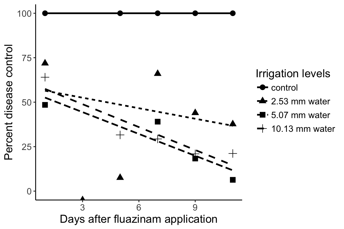

Additional visualizations

When we plot the averages, we inadvertently hide the data. Of course, if we tried to plot all the data in one graph, it would look a bit messy:

> ggplot(percents, aes(x = DAI, y = Area, group = Treatment)) +
+   geom_point(aes(pch = Treatment), size = 3) + # plot the points
+   stat_smooth(aes(lty = Treatment), method = "lm", se = FALSE, color = "black") + # plot the regression
+   theme_classic() + # change the appearance
+   ylim(0, 100) + # set the limits on the y axis
+   theme(text = element_text(size = 14)) + # increase the text size
+   labs(list( # Set the labels
+     x = "Days after fluazinam application",
+     y = "Percent disease control",
+     pch = "Irrigation levels",
+     lty = "Irrigation levels"))

Warning: Removed 41 rows containing non-finite values (stat_smooth).

Warning: Removed 40 rows containing missing values (geom_point).

Warning: Removed 80 rows containing missing values (geom_smooth).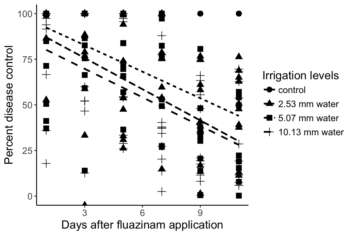

With ggplot2, we can spread the data out into “facets”:

> ggplot(percents, aes(x = DAI, y = Area, group = Treatment)) +
+   geom_point(aes(pch = Treatment), size = 2) + # plot the points
+   stat_smooth(aes(lty = Treatment), method = "lm", se = FALSE, color = "black") + # plot the regression
+   theme_classic() + # change the appearance
+   ylim(0, 100) + # set the limits on the y axis
+   theme(text = element_text(size = 14)) + # increase the text size
+   facet_wrap(~Treatment, nrow = 1) +
+   theme(aspect.ratio = 1) +
+   labs(list( # Set the labels
+     x = "Days after fluazinam application",
+     y = "Percent disease control",
+     pch = "Irrigation levels",
+     lty = "Irrigation levels"))

Warning: Removed 41 rows containing non-finite values (stat_smooth).

Warning: Removed 40 rows containing missing values (geom_point).

Warning: Removed 80 rows containing missing values (geom_smooth).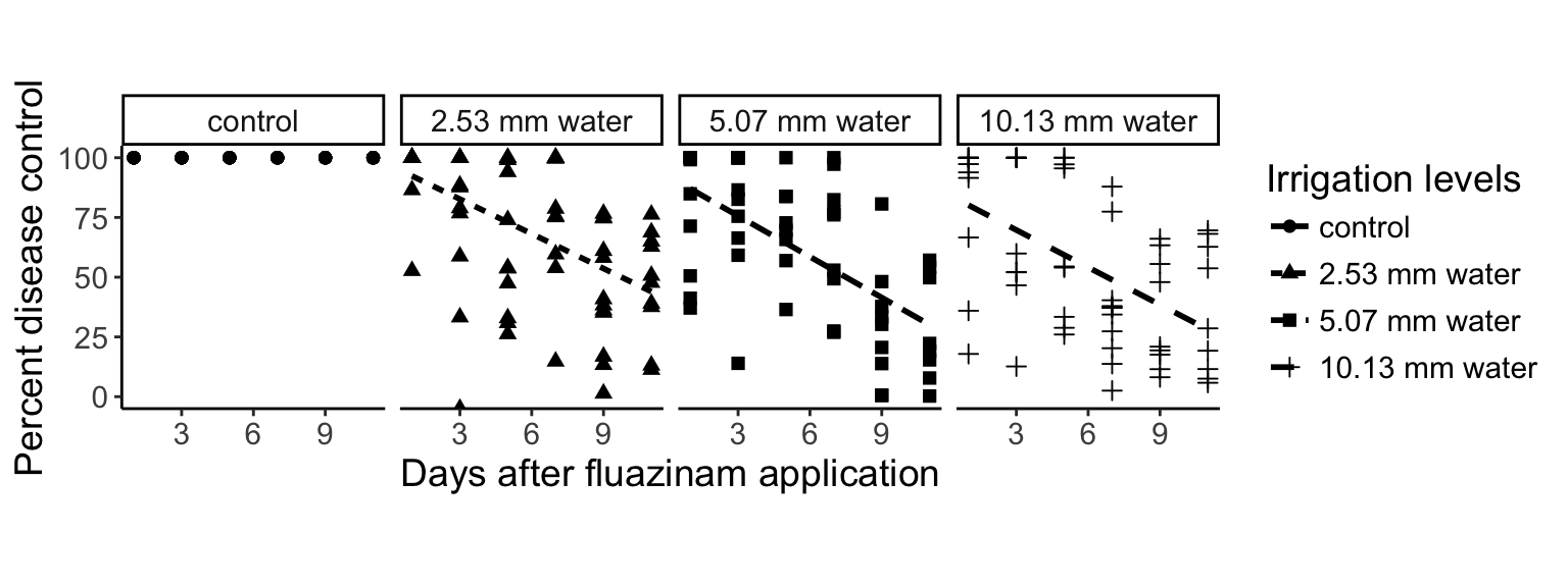

This work is licensed under a Creative Commons Attribution-ShareAlike 4.0 International License.